Much of the difficulty of training a neural net depends on the shape-related properties of the loss landscape, which can be related to network architecture and other optimization hyperparameters. But, because it is so high dimensional, it is hard to visualize or reason about. This paper offers a way of visualizing the loss landscape in a neighborhood around a local minimum, in such a way that these properties are better preserved.

• The paper proposes filter[-wise] normalization, which is a way of sampling local 2D neighborhoods around local minima such that the loss function can be plotted as a surface.
• The naive way to plot such a neighborhood would be:
  • Optimize the model to a local minimum with parameter vector \(\theta^0\), which is essentially a collection of weight matrices, one for each layer of the neural net.
  • Choose two random points \(\theta^1\) and \(\theta^2\) in a neighborhood around \(\theta^0\) as a basis¹¹In the paper’s notation, these are \(d_1\) and \(d_2\)., and generate a grid of affine combinations with them.
  • Plot the loss at high resolution in this 2D space.
• The trick is choosing how far away the 2 random points are, taking into account scale invariance of the weights due to batch normalization. If they are too close, it may appear to be too smooth. If too far, then too sharp.
• To get around this, for each random direction they normalize each “filter” in each layer to be equal to the original, like so: \[ \theta^k_{i,j} \leftarrow \frac{ \theta^k_{i,j} }{\|\theta^k_{i,j} \|} \|\theta^0_{i,j}\|, \] where \(\theta^{k=1,2}_{i,j}\) are initially Gaussian random points centered on \(\theta^0\), \(i\) indexes the layer, (where we are taking each weight matrix to be a “layer”,) and \(j\) indexes the “filter”, which is either a row or column, depending on whether the weight matrix is applied to input activations as a left- or right- multiplication.
  • What is this “filter” they keep talking about? It means the same thing as “neuron” or “unit”, i.e. a row or column of a weight matrix that produces a single scalar output activation. In convolutional layers it means “kernel” or “channel”.
• From this we can see that it’s not just a question of “how far away” each point \(d\) should be, but there’s also a kind of “shear” that has to be normalized out as well.
• Using this, they extract several insights:
  • The sharpness of local minima correlates with generalization error when the filter normalization is applied²²Cf. this paper, which shows that this is not true in general:
    Sharp Minima Can Generalize For Deep Nets
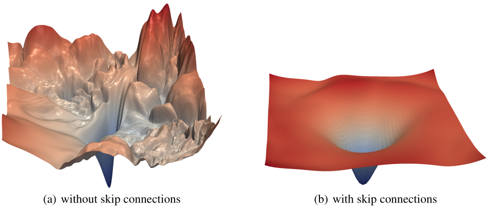
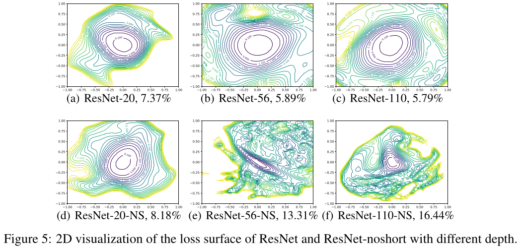
    Dinh et al. ICML 2017.
  • Deeper models (i.e., more layers) have more rugged loss landscapes, unless they have skip connections, which offers a suggestion as to why the skip connections help with generalization.
  • Wider models (i.e., more conv filters) have smoother loss landscapes.
  • Sufficiently deep DNNs show a kind of “phase transition” from smooth to highly non-smooth local neighborhoods.
  • In the settings that were studied, SGD trajectories fell within a low dimensional subspace.

• Clearly, weight magnitude and weight decay are confounded with the meaning of a “local” neighborhood, and if the wrong neighborhood is chosen then “sharpness” will be ill-defined.
• They also considered whether these 2D plots are representative of the higher dimensional space. Basically, if there is non-convexity in the 2D plot, then there definitely is non-convexity in the full dimensional neighborhood. Conversely, if there is none in the 2D plot, then probably there is little or none in the full dimensional neighborhood.

• The problem that this paper solves is that when plotting a 2D neighborhood around a local minimum \(\theta^0\), we might be “zoomed in” too close or too far to make a comparison.
• Since this paper, several others have noticed phase transitions in learning and related that to the statistical mechanics of SGD, especially “double descent” and even “triple descent”.
• It’s interesting to get a slightly better handle on when flat minima correlate with generalization accuracy, since the Dinh et al. paper shows that’s not always the case.
• By carefully choosing the size of a perturbation, they are really trying to determine what is a “meaningful perturbation”, which is a fairly deep question.
• This is similar, but not quite exactly the same, as other problems that can be reduced down to a single free parameter where one finds that ones hasn’t reduced the problem at all. For instance, a classifier with just one parameter \(\beta\) can have infinite VC dimension if it has the following form: \[ f(x) = \sin(\beta x) \]

Comments can be left on twitter, mastodon, as well as below, so have at it.

New post!

Paper outline: Visualizing the Loss Landscape of Neural Netshttps://t.co/UlblFSkB9K

Reply here if you have comments.

— The Weary Travelers blog (@wearyTravlrsBlg) June 25, 2023

To view the Giscus comment thread, enable Giscus and GitHub’s JavaScript or navigate to the specific discussion on Github.