Sharp Minima Can Generalize For Deep Nets

“Dinh et al., ICML 2017”

Following the trend of our earlier post on Visualizing the loss landscape, we’ll continue to look at how the loss landscape of neural nets affects their generalization properties.

Summary

There is a growing consensus that flat minima seem to correlate with better generalization¹¹Better generalization doesn’t necessarily better accuracy, just less gap between train and test error., so we should be looking for flatter minima, right? The paper shows that while there is something to this idea, it’s very easy to fool yourself. The way they show this is by giving examples of re-parameterizations of neural nets that compute the same function, and yet which have different degrees of sharpness around their minima. In particular, they show that (at least with ReLU units) the minima can be made sharper just by re-ordering the units.

What does “flatness” even mean?

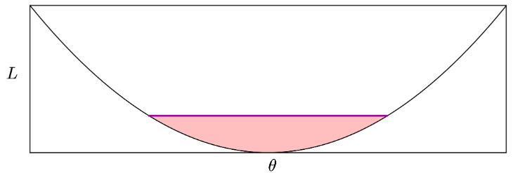
There are several ways of measuring flatness, and the paper breaks them into two broad categories. If we fix some constant \(\epsilon\), then it can either represent:

The size of the neighborhood having loss with \(\epsilon\).
The magnitude of the largest loss function value in an \(\epsilon\) -ball neighborhood.

In other words, “sharpness” is the height of the pink part of the figure, and “flatness” is the width, if the width or height are constant, respectively. The “sharpness” can also be related to eigenvalues of the Hessian.

A neat reparameterization trick

The paper then shows a neat trick that applies to ReLU neural networks. If I have two weight matrices in succession, \(\theta_1\) and \(\theta_2\), then scaling one by a factor \(\alpha\) is equivalent to scaling the next one by \(\alpha\). \[ \mbox{ReLU}(x^T(\alpha\theta_1))^T \theta_2 = \mbox{ReLU}(x^T\theta_1)^T(\alpha\theta_2) \] This ignores the bias term \(b_1\), but it’s easy to see that this trick still works when there is a bias. So the first symmetry that we see is that for any successive layers we can take any \(\alpha > 0\) times the first one and \(1/\alpha\) times the second one, and get an identical model, but one having a very different neighborhood.

Some results

Flatness is meaningless

The paper uses this trick to show that for a 2-layer MLP, the “flatness” of the above definition is always infinite. The argument works by showing that around every local minimum \(\theta\) there is a non-zero rectilinear \(\ell_\infty\) norm ball \(B_\infty(r, \theta)\) of size \(r\) that fits within the flatness region for some \(\epsilon\). Using the \(\alpha\) trick, we can map every point in \(B(r, \theta)\) to a new point \(T_\alpha(B_\infty(r, \theta))\), where \(T_\alpha\) is the \(\alpha\) trick expressed as a linear operator. There are infinitely many such mappings of \(B_\infty(r, \theta)\), they ’re all in the flatness region, and we can still find infinitely many that don’t overlap, so the measure of the flatness region is infinite.

The consequence of this result is that every local minimum is part of an infinite “level set” wherein the model’s output does not vary, meaning that “flatness” has no useful meaning and cannot be related to generalization.

Sharpness is meaningless

Some people also like Hessians, and for them the paper has another result showing that you can manipulate the trace and spectral norm²²Trace is the \(\ell_1\) norm of eigenvalues, (if they’re all nonnegative,) and Spectral norm is the \(\ell_\infty\) norm. Since we’re talking about Hessians of local minima, they are always positive semidefinite. of the Hessian however you like without changing the model’s prediction. This means that for any local minimum \(\theta\), you can find an infinitely sharp direction meaning that every \(\theta\) is infinitely sharp. The argument works by showing that the Frobenius norm of the Hessian of \(T_\alpha(\theta)\), where \(T_\alpha\) is the \(\alpha\) trick, is lower bounded by \(\alpha^{-2}\gamma\) where \(\gamma\) is a nonnegative term related to some arbitrary element of \(\theta\). Since we can pick any \(\alpha\) we want, we can make the sharpness whatever we want.

My observations

As with the Visualizing the loss landscape paper, when discussing or reasoning about smoothness of the loss landscape there is an extra degree of freedom controlling the scale³³That is, if you’re zoomed way in, anything looks flat. If you’re zoomed way out, anything looks sharp., and if it’s not controlled then the result may not mean what it seems to.

This paper goes beyond that and also tackles, or makes a start at tackling, another serious problem – accounting for the symmetries inherent to Deep Nets. It’s vogue now, (deservedly so, IMHO,) to say that classical statistical learning theory has no traction on neural nets, but it should be remembered that we can’t say affirmatively how wrong those theories are until we know they are being applied correctly. To be specific, the VC dimension idea is to establish a cardinality of the search space of functions, and then compute what amounts to Multiple Testing corrections for them. Well, how do we know what that theory even says if we don’t know that cardinality, and how do we know that cardinality if we’re only scratching the surface of symmetries between neural nets?

On the other hand, the paper doesn’t seem to offer any tricks to control for this variation the way the Visualizing the loss landscape paper did, meaning it’s kind of a negative result – that pure flatness / sharpness alone are essentially meaningless. It’s a bit disappointing that the paper doesn’t propose a refinement to the ideas of sharpness and flatness that quotients out the effect of parameters on model outputs, i.e. sharpness should be invariant wherever model outputs are invariant. Given that they’ve correlated with generalization in the past, there must be some way of defining a “canonical form” out of all the equivalent models that one can get, and then relating generalization to the canonical forms. But, the paper seems to have left that for a future work.

Thanks for reading to the end!

Comments

Comments can be left on twitter, mastodon, as well as below, so have at it.

New post!

Paper outline: Sharp Minima Can Generalize For Deep Netshttps://t.co/vtARFjVYF9

Reply here if you have comments.
— The Weary Travelers blog (@wearyTravlrsBlg) September 18, 2023

To view the Giscus comment thread, enable Giscus and GitHub’s JavaScript or navigate to the specific discussion on Github.

Footnotes:

Better generalization doesn’t necessarily better accuracy, just less gap between train and test error.

Trace is the \(\ell_1\) norm of eigenvalues, (if they’re all nonnegative,) and Spectral norm is the \(\ell_\infty\) norm. Since we’re talking about Hessians of local minima, they are always positive semidefinite.

That is, if you’re zoomed way in, anything looks flat. If you’re zoomed way out, anything looks sharp.