As the title suggests, there is a known interaction between Learning Rate and test accuracy; and there is also a known interaction between Batch Size and test accuracy. This paper offers a constructive way to convert between the units of one and the units of the other. Why should anyone care? Because larger batches are easier to parallelize and therefore offer a greater speedup. Hence, the paper title¹¹…assuming one is in a position to take advantage of the gargantuan batch sizes examined in this paper..

• How did this paper get at such a conversion?
  • The paper imports a result from an earlier paper²² A Bayesian Perspective on Generalization and Stochastic Gradient Descent
    Samuel Smith, Quoc Le
    Arxhiv 2017: \(g = \epsilon\left(\frac N B - 1 \right)\) where,
    • \(g\) is the scale of the stochastic fluctuations in the gradient, due to the stochasticity of using random batches
    • \(\epsilon\) is the Learning Rate
    • \(N\) is the size of the entire training set
    • \(B\) is the Batch Size
  • Note that where \(B = N\) the stochasticity goes to \(0\) as we would expect.
  • Also note that the Learning Rate linearly scales this stochasticity, also as we would expect.
  • Finally note that \(\epsilon\) and \(B\) contribute inversely to one another.
• Taking advantage of this trick is very easy. Any time you increase the batch size, just increase the learning rate by a similar factor, maintaining the proportion \(B \propto \epsilon\). That is, \[ \epsilon\left( \frac N B - 1 \right) \sim K \epsilon \left( \frac{N}{K B} - 1 \right), \] where \(K\) is the factor by which we can increase the batch size while still capturing a speedup.
• This paper also finds a relation between the momentum term \(m\) and \(B\): \(B \propto 1/ (1 - m)\). However they find the test accuracy is not as equivariant to this proportion as the one between \(B\) and \(\epsilon\). A momentum term really just implies a non-uniform averaging of gradients, so it shouldn’t come as a surprise that there is an effect related to it.
  • The generalized relation incorporating momentum is, \[ g = \frac{\epsilon}{1 - m} \left( \frac N B - 1\right) \]
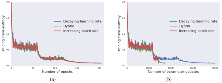
• Experiments on CIFAR-10 and ImageNet show that with this trick, the loss curves for equivalent learning rate and batch size schedules do indeed match one another very closely – so long as they are plotted per epoch, (i.e., the left side of the figure above). When the differences in Batch Size take effect, however, there are many fewer gradient updates per epoch, so the large batch sizes will get to the same minimal error in a lot fewer steps, (i.e., the right side of the figure above.)
• The paper tries this with several variants of SGD: with regular momentum and Nesterov momentum, and with Adam, and in all cases the proportional equivariance of \(B\) and \(\epsilon\) holds up very strongly.
• There is an important caveat here – this only holds up where \(B << N\). For CIFAR-10, with a training set of \(50,000\), they limited themselves to… \(5120\), for some reason. On ImageNet, with its 1.28M training images, they started with a batch size of 8192 and worked up all the way to \(81,920\). (For some reason, they later refined their method and the max Batch Size went back down to \(65,536\).)

• This paper’s main result comes from an earlier paper by the first and last authors²² A Bayesian Perspective on Generalization and Stochastic Gradient Descent
  Samuel Smith, Quoc Le
  Arxhiv 2017, which itself is based on a whole body of physics learning theory literature that is mostly based on the remarkable similarity between Stochastic Gradient Descent, which has this update form: \[ w_{t+1} - w_t = - \epsilon \nabla L_t + e, \] and the Langevin equation, which has this form: \[ \frac{d w}{dt} = - \lambda \nabla E + \eta(t). \] In both equations, \(w\) is a state vector. Both equations feature a gradient of something smooth and non-convex, with a scale factor – a Loss function \(L\) and \(\epsilon\) in the first, and a [Free] Energy function \(E\) with a damping coefficient \(\lambda\) in the second. Lastly, they each feature a kind of residual error term.

  The physics people usually adopt an i.i.d. noise model, which they write as, \[ \langle \eta_i(t) \eta_j(t') \rangle = 2\lambda k_B T \delta_{i,j}\delta(t - t'), \] where \(k_B\) is the Boltzmann constant, \(T\) is the temperature of the system and the \(\delta\) s indicate that there is \(0\) correlation between any \(i\) and \(j\), or between any \(t\) and \(t'\)³³Technically, something can still be statistically dependent while still being uncorrelated, but I’m not aware of anyone using this fact.. Incidentally, this equation appears on page 2 of the paper, but they don’t mention the connection with the Langevin equation. They do describe a relation to Simulated Annealing.

  In any case, the earlier 2017 paper by Smith and Le only mentions this fact in their Appendix A, but that is nevertheless where this result comes from.

  The paper that seems to have introduced this idea to the computer science world was this one⁴⁴ Bayesian Learning via Stochastic Gradient Langevin Dynamics
  Max Welling, Yee Whye Teh
  ICML 2011
  See our outline of this paper. by Max Welling and Yee Whye Teh. This paper uses the term “Langevin” in the title, and throughout.

• The paper mentions that they can train a ResNet to \(76.1\%\) in “under 30 minutes”, and oh by the way they were using a massive cluster of TPUs at google.
• For reasons that aren’t quite clear, they still need to start with smaller batch sizes and then increase them. Apparently there are numerical instabilities that limit how high the absolute learning rate can be and they just seem to take it for granted that while there is a strong equivariance between \(\epsilon\) and \(B\), it only holds for certain values of \(\epsilon\).

Comments can be left on twitter, mastodon, as well as below, so have at it.

New post!

Paper outline: Don’t Decay the Learning Rate, Increase the Batch Sizehttps://t.co/QhMzz967sd

Reply here if you have comments.

— The Weary Travelers blog (@wearyTravlrsBlg) July 23, 2023