

Deep Residual Learning for Image Recognition
This is the ResNet paper. As of December 2022, this paper has over 144K citations (up from 124K last I checked). If you’ve been doing machine learning with DNNs at all these last several years, it’s hard to imagine not having heard of ResNets. This paper has it all: a good motivation, a solid explanation as to why this works – even contrary to some common intuitions – and most of all, it has one of the strongest slam-dunk experiments sections I’ve ever seen. If you need a refresher on 2D convolutions, checkout these visualizations. 1Note that what’s shown there is done independently for each output channel, and, all input channels contribute to the output. Another fact that may be useful staying oriented – a \(1\times 1\) convolution on a 1 pixel image of \(c_{in}\) channels with \(c_{out}\) output channels is logically equivalent to a \(c_{in} \times c_{out}\) Fully Connected (FC) layer. A \(k\times k\) convolution on a padded \(h\times w \times c_{in}\) image will produce an \(h\times w \times c_{out}\) output image, and is equivalent to summing the output of \(k*k\) separate \(c_{in} \times c_{out}\) FC layers, each of which takes input from one of the \(h*w\) pixels.
Let’s dig in!
Summary
The paper sets itself the task of figuring out how to make Deep networks Deeper. The intro dismisses the old bugbear of Vanishing / Exploding gradients since the proper forms of normalization had been discovered. Instead, the paper makes an observation that’s been sitting in plain sight, but which goes against several common intuitions.
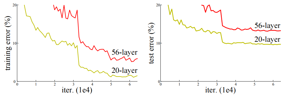
When deeper networks start converging, a degradation problem has been exposed: as the network depth increases, accuracy first gets saturated (which might be unsurprising) and then degrades rapidly. Unexpectedly, such degradation is not caused by overfitting, and adding more layers to a suitably deep model leads to higher training error
[emphasis original]
In other words, a certain dogma says “More layers, more capacity, higher training accuracy, more overfit” and this paper says, “Actually no!”
Instead of attacking the problem in terms of managing model capacity, this paper looks at another problem altogether: difficulty in optimizing the model. That is, if your model isn’t even realizing the capacity it has in theory, then there’s no use in trying to manage or control it. This points to a real problem – how many papers from before 2016 can you think of that explored architectures with over 100 layers? 2That is, from the current generation of DNNs. Apparently Jurgen Schmidhuber was experimenting with over 1000 layers in 1993.
The paper examines the declining training accuracy phenomenon in light of a simple thought experiment: what would happen if one were to set the later layers exactly equal to the Identity transform? Of course this would always have equal training and test accuracy. Yet, the above plot shows that for some reason the solvers are converging to something worse as models have more and more layers. The paper reasons that declining train accuracy is therefore not intrinsic to deeper nets, but rather an artifact of the optimization characteristics resulting from architecture choices. This thought experiment led to the core idea of the paper: adding skip connections, which the paper calls “shortcut connections”.
Let us consider \({\cal H}(x)\) as an underlying mapping to be fit…, with \(x\) denoting the inputs… If one hypothesizes that multiple nonlinear layers can asymptotically approximate complicated functions, then it is equivalent to hypothesize that they can asymptotically approximate the residual functions, i.e., \({\cal H}(x) − x\)… So rather than expect stacked layers to approximate \({\cal H}(x)\), we explicitly let these layers approximate a residual function \({\cal F}(x) := {\cal H}(x) − x\). The original function thus becomes \({\cal F}(x)+x\).
With skip connections, the output of each layer is a delta between the previous layer and whatever the expected output is, which is the definition of a residual. This way, if the model can’t find a no-op on its own, then at least we could try to make it easier to find one – by giving quiescent residuals. Hence, ResNet.
The central proposition of the paper is the residual unit, a combination of convolutional layers with a pass-through connection (the identity transform from the thought experiment), which they later refine into the bottleneck unit.
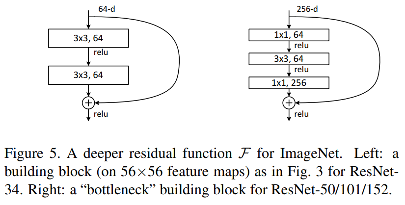
In practice, the residual units (left), tend to be about as common as bottleneck units (right, described below).
ResNet architecture
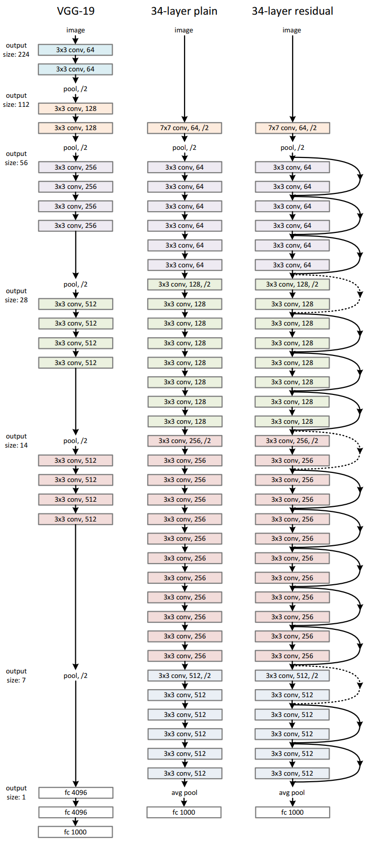
The proposed architecture starts with a single \(7\times 7\) convolution, and then adds lots of residual units in sequence, followed by a single FC layer for the classification. This diagram compares ResNet-34 against the VGG-19 model, (so named because it had only 19 layers total,) which is a standard convolutional net with just lots of layers and pooling, plus 3 large FC layers at the end. ResNet itself has only two pooling steps, 3 strided convolutions, and a single FC layer at the end. With this general architectural approach, the paper considers versions of it having 18, 34, 50, 101, and 152 layers. That’s individual layers, not residual units, each of which is 2 layers, or bottleneck units, which are 3.
Without the residual units, i.e. with a plain convolutional architecture and no skip connections, the 18 layer model gets about a 28% top-1 error on ImageNet. Top-1 error goes up by half of a point with 34 layers, which is probably significant, but the paper doesn’t say. However, when using residual units instead, it gets the same roughly 28% at 18 layers, but then its error goes down to 25% at 34 layers. And there you have it – more depth leads to better accuracy.
To underscore that this isn’t just a cherry-picked point estimate, the paper shows some error curves that show that train and test error decreasing between the 18 and 34 layer ResNets, but increasing between the 18 and 34 layer plain convolutional nets.
One very interesting aspect of their architecture is that although the ResNet has roughly double the number of conv layers as VGG-19, (16 vs. 33), it works out to only 18% of the FLOPs of VGG-19 on a forward pass. This is because VGG-19 rapidly increases the number of channels per layer, and hence uses its capacity in a less efficient way. Meanwhile, ResNet increases the channel-width slowly over a greater number of layers, and drops the massive \(4096\times 4096\) FC layers at the end. Hence, in spite of being substantially deeper, it is a lot less compute intensive.
As we’ll see, the authors chose to reinvest the savings in… more layers.
So far so good, but there’s just one problem: What do we do when the number of channels changes, e.g. from 64 to 128? We can’t just add the residual to the previous layer’s output when they have different dimensions. The paper suggests 3 approaches for dealing with such cases:
- 0-pad the extra channels when increasing their number.
- Use \(1\times 1\) convolutions, i.e., \({\cal F}(x) := {\cal H}(x) - Conv_{1\times 1}(x)\), only when the number of channels changes
- USe \(1\times 1\) convolutions, but for all skip layers.
The paper’s experiments show that in a 34 layer model the third option (24.2% top-1 error) is slightly better than the second (24.5%), which is slightly better than the first (25.0%). The main point, however, is that whatever approach is taken, the skip connections and added depth do most of the lifting, compared with the original 28% top-1 error without them.
The third option might seem a bit strange – why would we add an extra \(1\times 1\) convolution when we are supposed to be learning only the residual function? That is, we’re trying to learn \({\cal F}(x) := {\cal H}(x) - x\) so that in case \({\cal H}(x)\) is not learnable from the features \(x\), \({\cal F}\) can just be a \(0\) function, which is learnable. Yet, the experiments above show that it is slightly better. I think this means two things –
- A \(1\times 1\) convolution doesn’t necessarily change the total information content of a pixel, so long as it’s full rank and reasonably well conditioned.
- Perhaps a Deep Net benefits slightly from letting the information content of its channels mutate from one layer to the next; if all we do is learn residuals, then the model is stuck with whatever channels are learnt at the bottom end, closest to the data. If there is a more useful recombination of the channels, then this architecture may not be able to learn it as readily.
The paper also makes an intriguing comment in passing:
The form of the residual function \(\cal{F}\) is flexible. Experiments in this paper involve a function \(\cal{F}\) that has two or three layers (Fig. 5), while more layers are possible. But if \(\cal{F}\) has only a single layer, Eqn.(1) is similar to a linear layer: \(y = W_1x + x\), for which we have not observed advantages.
In other words, in order to really benefit from the residual trick, you have to learn a nonlinear residual. That is, the information used to correct the error of \(x\) has to undergo several convolutions on its own before rejoining, or else it won’t add much value, if any.
There is one caveat to this, which will matter more later – at large numbers of channels, even \(1\times 1\) convolutions can be
surprisingly expensive. Each one is essentially an FC layer that operates in parallel on every pixel. Its
parameter tensor is \(k_h \times k_w \times c_{in} \times c_{out}\), so a \(1\times 1\) from \(256 \to 256\) has 65,536
parameters, and each pixel at that level needs the equivalent of a \(256\times 256\) matrix multiply. Given that, from a
compute ROI perspective, there does eventually come a point where the extra \(1\times 1\) convolution from option 3 above
doesn’t provide any further value over option 2, which was slight in the first place. The paper says that apart from the
34 and 50 layer ResNets they didn’t pursue the third option, and used the second instead. This also matters for the
bottleneck units.
Bottleneck units
The paper then introduces bottleneck units, which leverage another important observation. The idea of a bottleneck
unit is that the residual is computed at a lower channel resolution, and then projected back up to full resolution.
(Channel resolution, not spatial.) This forces it to choose what information it wants to use first, essentially
compressing it first, before fitting the residual. For example, say layer l outputs 256 channels. The bottleneck
comprising layer l+1 consists of a \(1\times 1\) convolution that first reduces them by 4x to only 64 channels. Then a single
\(3\times 3\) is applied to compute the residual. Then, yet another \(1\times 1\) is applied, bringing the channels back up to 256,
whereupon the decompressed residual is summed with the skip connection and the nonlinearity applied.
This is a rather clever thing to do. Consider that the \(1\times 1\) \(256\to 64\) conv loses information, which the \(1\times 1\) \(64\to 256\) conv cannot replace, but not to worry, any information that was lost is still there in the skip connection. It also massively reduces the compute load: at 256 channels, compared with a single \(3\times 3\) convolution, the bottleneck unit lowers the compute time and parameter count by about 9x!3That is, between the \(1\times 1\) down, the \(3\times 3\) at lower resolution and the \(1\times 1\) up, \(256\times 64\) + \(9\times 64 \times 64\) + \(64 \times 256 = 69,632\) parameters, vs. the \(3\times 3\) at full resolution which has \(9\times 256 \times 256 = 589,824\)! Since convolutions are linear operations, parameter count is a reasonable proxy for compute load.
Whether you believe there’s a regularization win from forcing it to compute the residual under compression, or that the compute savings can be reinvested into more layers, which is just better, (or both,) this trick really works. Ramping up to 152 layers still only brings it to 11.3G FLOP, compared with VGGNet’s 19.6. Using this trick gets yet another 6 % points (19.4%). They have now gone from 28.54% top-1 error to 19.38% on ImageNet.
It’s not often that one can apply one simple trick to reduce SOTA error by several whole % points, and then do it again with another.
Further experiments on CIFAR
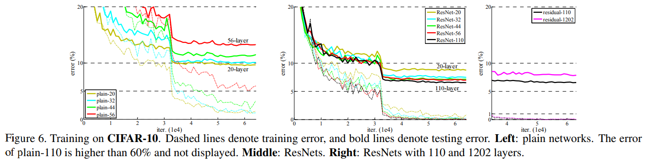
Having demonstrated superiority on ImageNet, the paper is still relentless about searching for an understanding of why this trick works, rather than just accepting that something they threw at the wall stuck. To get at some of these questions the authors ran more experiments on CIFAR-10. Since CIFAR-10 is much smaller, they can try more things, meaning they can, or could have, explored even deeper models. For some reason, they ran CIFAR experiments at 20, 32, 44, 56, 110 layers, and… 1202. Of that set, 110 was the best. Why didn’t they do 150, or 300? Who knows. But at least they went for something truly bananas like 1202.
As with ImageNet, they provide error curves once again showing that as depth increases from 32 to 56, error decreases for the ResNet, but it increases for the plain convolutional net. That is, except for the 1202 layer ResNet, which has higher test error. The paper points out that with more and more layers of depth there has to be a point where more regularization is needed, and eventually it gets there.
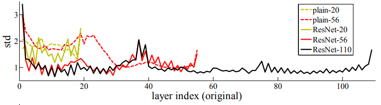
Activation variance
The paper surmises that since more layers means more accuracy, each successive layer should be producing a more accurate output, and hence the residuals should be getting quieter. What’s actually happening is… more complicated. Some of it looks like a kind of resonant pattern or Gibbs ringing, but there is a trend with deeper nets towards lower activity overall. See for yourself.
So that’s the paper. What did I take away from it?
- It’s hard to overstate how important that initial insight is – that adding more layers to a network doesn’t just magically give it more capacity. Capacity isn’t just a function of the architecture, but also the preprocessing, and optimization too. For instance, by carefully normalizing the data or fine-tuning the learning rate schedule one can coax a DNN into getting near-perfect training error4Training error decreases as model capacity increases. Once it hits 0 on one dataset, one would need a larger / harder dataset to observe further increases in capacity. on larger data sets. The paper does more than just provide an insight, however – it actually makes it useful.
- In this paper, skip connections were thought of as a way of fixing something broken about the models to see if they could make a thought experiment came out as expected. The fact that they might have actually improved training error and generalization was total serendipity! This is why it’s important to always build a toy model to try to fix or control something that doesn’t make sense.
- Interestingly, they point out that the 2015 Inception paper5Going Deeper with Convolutions
Szegedy et al. CVPR 2015 had skip layers leading directly to a separate classification / loss term that was discarded at inference time, that was explicitly intended as a fix for exploding and vanishing gradients. This is telling – it suggests you can’t climb the next hill as long as you’re struggling with the current one. Several other papers came close to making the same discovery, but they either made their use of skip connections too complicated with e.g. gating functions, or else they only added skip connections from the input layer, and not elsewhere throughout the network. - The paper demonstrates in several ways that there are better and worse ways of investing a compute budget. Where it really shows is in the channel width of the convolutions, and they are judicious about raising the channels or not using them frivolously, e.g., in the \(1\times 1\) convolutions on the skip connections. The purpose of all of the frugality, though, is really to enable them to add more layers.
- One possible reason why the model can’t find the identity transform on its own could be because the identity is a
very sparse pattern. In order for a model to settle on such a sparse pattern it would be necessary6Technically, there is a 0-measure set of non-sparse gradient updates that would accomplish this, but it’s not
clear whether any error term at the head could produce such an effect at more than one layer., but not
sufficient, to have a sparse gradient, and that is clearly not happening on its own. The skip connection trick
bypassed the problem altogether by changing variables such that the same no-op pattern is not sparse, but just
extremely low mean / low variance, which SGD can find by itself. But what if there are
other sparse patterns7The Lottery Ticket Hypothesis: finding sparse, trainable neural networks
Frankle, Carbin ICLR 2019 waiting to be discovered? - The Gibbs-like effect in the activation variability per layer makes me wonder if there is some feedback happening. Consider that at each residual unit, every gradient step affects both the residual and the previous layer at the same time. This is bound to produce some double-correction, and where there is overcorrection there may be oscillation.
- To my eye looking back from 20228and now publishing in 2023…, Residual Units look a lot like a poor man’s
partial concept classes (PCCs)9A Theory of PAC Learnability of Partial Concept Classes
Alon et al. FOCS 2021. That is, the earlier layers learn the broad concept, and later layers are, if working as intended, only learning the exceptions, and then the exceptions to the exceptions and so on. Like partial concepts, exceptions are only defined in certain regions of latent space. Given the sparsity inducing behavior of ReLU units it’s conceivable that something sort of like this may be happening, but on the other hand given the variability in the activations per layer in the 110 layer ResNet, maybe something else is going on. - By now it’s pretty well known that the
teacher-student distillation model10Distilling the Knowledge in a Neural Network
Hinton et al. arxiv 2015, wherein one first trains a big complicated model, and then trains a single, simpler model using just the input/output pairs from the teacher model, is a very effective trick. In a way, this may be similar to what the bottleneck units are doing. That is, they have a source and a target, and they try to learn to update, but they have to mimic it at a lower channel resolution.
Final thoughts
It’s easy to think of this paper as a lab writeup on a new widget that wins contests easily, but I think a better way to read it is to see that, at least in this instance, you can win all of that fame and fortune by optimizing better. The widget isn’t for winning contests, or even improving generalization. It’s for improving the optimization. Who knows, maybe there are more ideas to be found by thinking of some obvious pattern that SGD ought to be able to find, but can’t, and then designing a widget to help it.
The Rich Sutton Bitter Lesson essay says, essentially, it’s a waste of time trying to encode beliefs directly into the loss function via some fancy regularizer, and that instead one should look for a framework that improves with more compute power, no matter how much one has. It uses the term “invariances” only once, but I think it’s the most critical word in the entire essay. Invariances are a kind of prior, but they aren’t facts or knowledge, they’re properties. They’re regularities. I think residual connections are a way of finding regularities in a much more compute-efficient way.
This paper11Visualizing the Loss Landscape of Neural Nets
Li et al., NeurIPS 2018
See our outline of this paper., and others, show that the loss landscape is impacted greatly, and positively, by the residual connections. By making
the loss landscape more regular they ensure that no small perturbation can radically alter the model’s training
accuracy, and that is the kind of regularity that really matters.
I also can’t help but notice that when done right, the total compute burden goes down, which may take some of the bitterness out of the lesson.
Thanks for reading to the end!
Comments
Comments can be left on twitter, mastodon, as well as below, so have at it.
New post!
— The Weary Travelers blog (@wearyTravlrsBlg) July 15, 2023
Paper review: The ResNet paperhttps://t.co/rSbpXk2cI6
Reply here if you have comments.
To view the Giscus comment thread, enable Giscus and GitHub’s JavaScript or navigate to the specific discussion on Github.
Footnotes:
Note that what’s shown there is done independently for each output channel, and, all input channels contribute to the output. Another fact that may be useful staying oriented – a \(1\times 1\) convolution on a 1 pixel image of \(c_{in}\) channels with \(c_{out}\) output channels is logically equivalent to a \(c_{in} \times c_{out}\) Fully Connected (FC) layer. A \(k\times k\) convolution on a padded \(h\times w \times c_{in}\) image will produce an \(h\times w \times c_{out}\) output image, and is equivalent to summing the output of \(k*k\) separate \(c_{in} \times c_{out}\) FC layers, each of which takes input from one of the \(h*w\) pixels.
That is, from the current generation of DNNs. Apparently Jurgen Schmidhuber was experimenting with over 1000 layers in 1993.
That is, between the \(1\times 1\) down, the \(3\times 3\) at lower resolution and the \(1\times 1\) up, \(256\times 64\) + \(9\times 64 \times 64\) + \(64 \times 256 = 69,632\) parameters, vs. the \(3\times 3\) at full resolution which has \(9\times 256 \times 256 = 589,824\)!
Training error decreases as model capacity increases. Once it hits 0 on one dataset, one would need a larger / harder dataset to observe further increases in capacity.
Going Deeper with Convolutions
Szegedy et al. CVPR 2015
Technically, there is a 0-measure set of non-sparse gradient updates that would accomplish this, but it’s not clear whether any error term at the head could produce such an effect at more than one layer.
The Lottery Ticket Hypothesis: finding sparse, trainable neural networks
Frankle, Carbin ICLR 2019
and now publishing in 2023…
A Theory of PAC Learnability of Partial Concept Classes
Alon et al. FOCS 2021
Distilling the Knowledge in a Neural Network
Hinton et al. arxiv 2015
Visualizing the Loss Landscape of Neural Nets
Li et al., NeurIPS 2018
See our outline of this paper.