

Neural networks and physical systems with emergent collective computational abilities
This one is even more of a throwback than our first review – it’s a 40 year old paper in PNAS by a neurobiologist. At first glance it may not seem all that central to the current wave of Deep Learning. Yet, at some point you’ve probably at least heard of Hopfield nets and the related Hebbian learning, which can provide a good parallax point for understanding modern Deep recurrent nets. This is the breakthrough paper that showed the idea might actually work.
The key to understanding Hopfield nets and Hebbian learning is that while modern DNNs are designed for approximating a functional relation between one domain and another, where the intention is to generalize and interpolate, Hopfield nets are intentionally designed as memorizers, where the intention is to only generalize up to a point. It turns out that there are a few very clever tricks underlying their ability to do so, and I have a feeling they will be rediscovered1By “rediscovered” I mean being cited the way mainstream DNN papers get cited. People are still publishing about them, but they’re nowhere near as well cited. sooner or later.
Let’s dig in!
Summary
This PNAS paper introduces Hopfield networks, a form of neural memory storage, which the paper calls “content addressable memory”2This differs somewhat from recent usage. Nowadays, “Content addressable storage” means that a cryptographic hash of the content is the key for its retrieval. The Interplanetary File System is a good example of this. This PNAS paper uses a different meaning – the retrieval key is a sufficient substring of the value, where “sufficiency” depends on the details of the implementation.. Observing that complex characteristics can arise emergently from many interacting simple agents, the paper asks whether some useful computational properties can be made to arise from a collection of simple neuron-like elements. The paper describes simulation experiments validating the error checking and recovery properties of these networks, and their various behaviors.
The Hopfield net is a different kind of neural net with a different purpose and radically different operating principles than standard feed-forward or recurrent networks. The purpose of a Hopfield net is to store and retrieve strings of bits that may have loss and / or corruption. The states are described by a vector of binary variables, and their transition function obeys an asynchronous evolution that has analogies to Ising models of magnetic spin systems. That is, rather than providing an input and feeding it forward synchronously all the way to the output, with or without recurrence, a Hopfield net operates by setting an initial state, and allowing the system to evolve asynchronously until it converges to a Fixed Point3I.e., a state that is its own successor.. That new state is the output.
Conceptually, if we want a robust retrieval property then for each desired “canonical” output there should be a set of similar, potentially “corrupted” or incomplete states that will map to it. This means that the “canonical” outputs need to be stable, while all others should be unstable, at least with high probability.
Update rule
How do we enforce such a property? The Hopfield network provides a weight update rule that ensures it. Concretely, the state space is described by \(N\) binary bits \(V_i\). The evolution function is described by a perceptron-like summation of a set of weights \(T \in \{0,1\}^{N\times N}\) connecting them, with a step-function nonlinearity. \[ \underset{V_i\to 0}{V_i\to 1} \qquad \mbox{if } \sum_{j\ne i} T_{ij}V_j \qquad \underset{< U_i}{> U_i } \] Note the very un-perceptron-like global recurrence implied here. So, in order to recover a pristine string \(V^* \in \{0,1\}^N\) that was actually stored, given some fragment or corrupted version of it \(\hat{V}\), we would set the state vector \(V_0 := \hat{V}\), and let the state evolve under this rule until it reaches a fixed point, which is hopefully \(V^*\).
That nonlinearity does something interesting - without it, the purely linear update rule at time \(t\) would be \[ V_{t+1} = \frac{T V_t}{\| T V_t \|} \] and the stable states would be exactly the eigenvectors of \(T\). If \(\tilde{V}\) isn’t an eigenvector, then it’ll asymptotically converge to the eigenvector \(v_i\) that maximizes \(\lambda_i v_i^T\tilde{V}\). It’s not very useful if one can only encode patterns that are strictly orthogonal to one another. With the nonlinearity, we can instead encode patterns with more flexibility - they simply have to be uncorrelated, which can be ensured with some pre-processing.
Storage
So we know how the Hopfield net retrieves stored patterns, but how does it store them? Suppose we have a dictionary of strings \(V^s \in \{0,1\}^N, s \in 1 \dots n\) that we would like to store. There just so happens to be an initialization rule that will enable this: \[ T_{i\ne j} = \sum_s(2V_i^s - 1)(2V_j^s - 1) \] The \((2V_i^s - 1)\) pattern is just converting \(\{0,1\}\) binaries into \(\{-1,1\}\) binaries4Alternatively, we can think of this rule as setting \(T_{ij}\) to be the number of patterns that are the same at \(i\) and \(j\) minus the number of patterns that are different.. From here out we also assume that \(T_{ii} = 0\) since whatever value \(T_{ii}\) has can instead be put into the threshold \(U_i\).
With that we can initialize \(T\), but how do we update it? We can assemble the \(0-1\) binary patterns \(V^s\) into a matrix \(D\) so that \(D_{\cdot s} = 2V^s -1\), which are \(\pm 1\) binary patterns. The rule can also be written as a sum of rank-one updates5A rank-one update is where we update a matrix \(T\) by adding to it another matrix \(M_1\) whose rank is one. Any rank-one matrix can be written as an outer product of two vectors, \(M_1 = vv^T\). Updating \(T\) by adding \(DD^T\) is equivalent to doing a series of rank-one updates. to \(T\), \[ T = \sum_s D_{\cdot s}D_{\cdot s}^T - n {\mathbf I} = DD^T - n {\mathbf I}, \] It follows that storing, or attempting to store, a single new pattern is also accomplished via a rank-one update.
With this update rule in hand, the recovery of \(V^s\) given some corruption \(\tilde{V^s}\) still requires \(V^s\) to be a stable state. How do we know that it is? When \(T\) is set as above then the evolution rule for a single element \(V_i\) is given as, \[ V_i \sim \sum_j T_{ij}V_j = \sum_sD_{i s} \left[ D_{\cdot s}^TV \right]. \] The term in square brackets is the inner product of pattern \(D_{\cdot s}\) with the current state \(V\). If \(V\) happens to be the same pattern as \(D_{\cdot,s}\), then the inner product of \(V\) with \(D_{\cdot, s}\) will be the number of ones in \(V^s\) – on the order of \(N/2\) – and all of the other inner products will be \(\sim 0\) – on average. If it is large, then the sign of \(D_{is}\) will determine the value of \(V_i\) at the next time step, which is to say, \(V_i\) will stay the same.
Unfortunately we don’t get a free lunch. All of this depends on that square-bracketed term being close to \(0\) for all of the other patterns that are not \(V^s\). So long as they are distributed more or less isotropically6Isotropy is the property that a set or distribution is spherically symmetric. This is synonymous with the axis variables \(V_i\) being uncorrelated., then it’s safe to assume so. Equivalently, if all of the \(i\) and \(j\) elements have low correlations across the dictionary then this will work. The paper argues that this is ok as long as we assume that some sensory subsystem has found an embedding for the patterns that has this property.
With this learning rule we always get a symmetric weight matrix \(T\), but that seems wasteful – half of the weights are redundant. Being symmetric gives \(T\) the useful property that it will be stable like we saw above, but there are also ways of setting \(T\) that aren’t symmetric. The problem is, sometimes those have stable cycles rather than stable states, and that is a whole other topic.
Hebbian learning
The model proposed in the paper is indeed novel, but it didn’t come out of nowhere. There were already several models trying to solve the same kind of problem, but they didn’t quite have the nice properties of storage and retrieval that this one does. One of the things they do have in common is that they have a similar update rule, which is the Hebbs rule, which the paper gives this form: \[ \Delta T_{ij} = [V_i(t)V_j(t)]_\mbox{average} \] with the average being taken over some windowed time series indexed by \(t\). Clearly it’s a sum of rank-one updates, just as this paper’s own rule is. The difference is, they’re not given explicitly as specific patterns, but as potentially noisy ones. In the Hebbian learning model, the states are potentially noisy, and the averaging attenuates that. Presumably they’re perturbed by specific patterns that an external system wishes to store, or to retrieve them, and otherwise keep evolving and updating on their own.
Statistical Mechanics and Energy Landscapes
Above we showed via plain linear algebra that when \(T\) is composed of rank-one outer products then those patterns are the stable points. But, there is another way to show this property, and it links Hopfield nets with statistical mechanics. It turns out that if we can define some “energy function” for each state, and if we can show that the evolution function never increases this energy function, then we know that any local minimum of the resulting energy “landscape”7Here, “energy landscape” means something like a Gibbs Free Energy or Potential Energy, which can be expected to decrease over time towards a local minimum. Depending on which statistical ensemble one uses to model the system, energy may or may not be locally conserved as it moves in or out of the system. is a stable state with high probability as desired, and will have an approximately convex local neighborhood.
This is more than what we knew before – the only thing we showed above was that the patterns \(V^s\) are stable. Now, according to the analogy from Ising models, we should see that the patterns that converge to \(V^s\) form a locally convex neighborhood. To do this we just need to create such an energy function, and the paper shows there is indeed such a function: \[ E = -\frac 1 2 \sum_{i,j} T_{ij}V_iV_j = V^TTV, \] and indeed the evolution step reduces it: \[ \Delta E = - \Delta V_i \sum_jT_{ij}V_j. \] This means that stable states are local minima, as desired. The paper says that this form is isomorphic to Ising Spin Glass models, which allows the application of a result from that theory stating that if \(T\) is symmetric and “random” then there will be “many” stable local minima to the above energy function, implying that this network will be able to store “many” points of data. But how many, and under what conditions?
Experiments
There were several aspects of the model that the paper examined experimentally. Since it was 1982, the paper only explored cases where \(N = 30\) and \(N = 100\), so there might be different results for higher parameter settings. Nevertheless, a biologically plausible model for simple ganglia in invertebrates would be for \(N\) in the range of \(100\) – \(10,000\), putting the experiments here on the lower end of that range.
Does it actually converge?
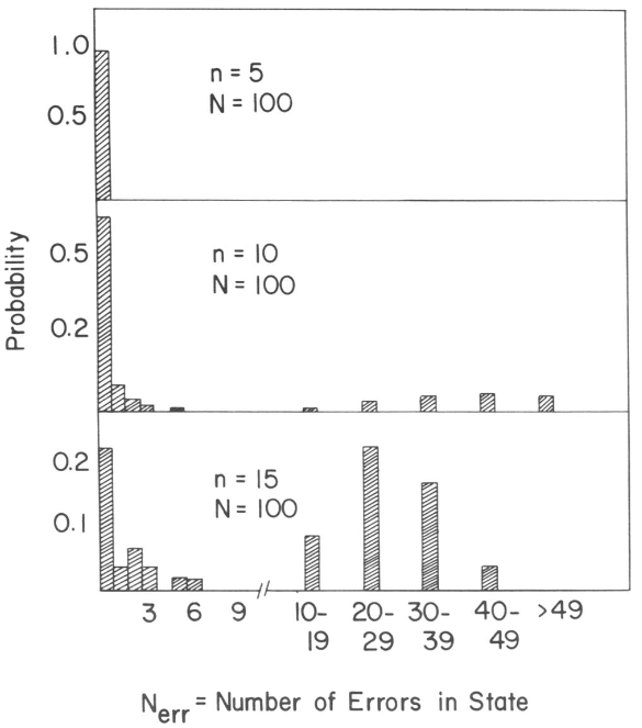
The short answer is, “usually”, and that’s assuming the network isn’t overloaded. (See below.) The first thing they tried was to encode some memories, and then feed it random \(\tilde{V}\) patterns to see where it ended up. With just 5 encoded memories, it tended to converge to one of them about 85% of the time, and 5% were near but not exactly on one of the patterns. If this were the hit rate for actual queries it would not be very good, but it shows that almost all of the state space is dominated by just the 5 patterns.
When there are more than 5 patterns, there tended to be more errors. With 15 patterns of \(N=100\) bits, there was about a 50-50 chance that a stable state would result having \(<5\) errors. This wouldn’t work as actual computer memory, but it’s potentially useful for some things.
Does the weight matrix have to be symmetric?
As mentioned above, the update rule proposed above always gives a symmetric \(T\). To see what happens when symmetry is broken, Monte Carlo experiments were done with \(N=30\) and \(N=100\). After initializing \(T\) as above, additional non-symmetric updates were made using this rule: \[ \Delta T_{ij} = A\sum_s (sV^{s+1}_i - 1)(2V^s_j - 1), \] where \(A\) is an adjustable rate. The paper found that this occasionally resulted in cyclical “metastable” configurations, one of which involved drifting back and forth between \(V^s\) and \(V^{s+1}\).
How many patterns can be stored?
Empirically, the paper found that about \(0.15N\) patterns or “memories” can be encoded with its update rule, and even then with a significant number of errors in retrieval. The probability of an error at a single bit is approximately Gaussian for large enough systems with enough memories stored in them:8Probably because of a Central Limit behavior. \[ P = \frac{1}{\sqrt{2\pi\sigma^2}} \int_{N/2}^\infty e^{\frac{-x^2}{2\sigma^2}}dx \] Note the integration from \(N/2\), so this is the area under one tail, where \(\sigma\) is the standard deviation given by \(\sigma \equiv [(n-1)N/2]^{1/2}\). This is the RMS error from the square-bracketed term in the derivation of the update rule. Increasing \(N\), i.e., making the net larger, will both move the tail further and increase \(\sigma\); increasing \(n\), i.e., adding more patterns, increases \(\sigma\) only.
Where \(n= 10\), \(N = 100\), \(P = 0.0091\), meaning that there is about a \(40\%\) chance that a pattern of \(N = 100\) bits will be recovered with no error. In simulations, however, it was \(0.6\).
Other interesting properties
- If a particular state is stable, then its ones-complement is also stable, so long as you use the paper’s update rule which keeps \(T\) symmetric.
- The state 00…00 is always stable, (under a 0-1 encoding), and with a uniform threshold on all neurons it is a low energy state meaning that mismatched queries will likely end up there giving it a “not found” interpretation.
- Individual memories need to be at least \(N/3\) to \(N/2\) Hamming units apart in order not to run into one another.
- Adding too many memories makes the system unstable and all of the previous memories are lost.
- This can be combated by clipping entries of \(T\) to a small value, e.g. 3, which permits more recent memories to be retrieved and older ones lost. The paper just says that a max of 3 is “appropriate” for \(N=100\).
- If we update \(T\) with only some \(k\) bits worth of information, then that sub-pattern will be stable, with the other bits being filled in with whatever they would have been, had that update not been made.
- Even if a net is grossly overloaded, (they tried \(5N\) patterns!) there is still a distinguishable pattern of state readjustments for previously seen examples being preferred over unseen ones. That said, none of the previously seen examples were stable, and this effect is only detectable at the population level.
- The tendency to arrive at stable states at or near the stored memories was fairly robust to variations in the details of the simulation.
So that’s the paper. What did I take away from it?
- I find it interesting that there is no need for noising or regularization because Hopfield nets don’t seek generalization, only robustness.
- Hamming codes can correct just one bit of error and detect up to two, at the expense of having \(\log_2 N\) more bits of information to transmit. Hopfield nets, on the other hand, can correct up to about \(N/3\) errors with high probability (at the \((N,n)\) point the paper simulated), and up to almost \(N/2\) with probability above chance, at the expense of having about \(1/0.15 \sim 6\times\) as many parameters as the data itself. Unlike Hamming codes, there’s no guarantee, only a probability.
- See also Viterbi decoders and Turbo codes.
- Being written by a neurobiologist, the paper makes a lot of motivating connections with the underlying physiology and architectonics of biological brains. A particularly interesting one is the observation that in cortical columns there are between \(100\) and \(10,000\) neurons. Since it was 1982, their simulations maxed out at about \(100\), but \(10,000\times 10,000\) is now a quite attainable size for a DNN module.
- Recently some papers have noticed that you can greatly reduce the number of floating point bits in some operators. Effectively this coarsely discretizes latent space – one of the pathological cases that adversarial attacks seem to exploit is narrow, sliver-like regions corresponding a single class, which are highly non-robust because a slight perturbation in some directions can move to an altogether different class, and a slight perturbation that does that is precisely an adversarial attack. I can’t help but notice that the strict binarization of the output of a Hopfield net is doing something similar, i.e. getting rid of small perturbations altogether.
- There is quite a bit of fiddling represented in this paper, some of which results in interesting properties. I definitely applaud the creativity shown in testing, e.g. the grossly overloaded setting with \(5N\) patterns, which would be a counterintuitive setting to explore after establishing that with only \(0.15N\) patterns they start to become unstable.
- There is something charming about a memory model that requires some “thinking” for a while that culminates in a retrieval of something previously seen, but with some potential for error. It certainly describes the user experience of human memory in some ways.
Final thoughts
This is a landmark paper that proved a concept – that self-updating systems can exhibit emergent memories. In terms of
raw performance it’s just ok, but then, most first prototypes usually are. There are several recent photonics papers
citing it9E.g.,
Photonics for artificial intelligence and neuromorphic computing
Shashtri et al. Nature photonics 2021
Inference in artificial intelligence with deep optics and photonics
Wetzstein et al. Nature, 2020, and Hopfield himself is still going strong10E.g.,
Large Associative Memory Problem in Neurobiology and Machine Learning
Krotov & Hopfield, arxhiv 2020
Bio-Inspired Hashing for Unsupervised Similarity Search
Ryali et al., ICML 2020
which shows that a) it’s still relevant and b) there’s still a whole other community outside of computer science
pursuing their own path to machine intelligence.
As a computer scientist, what I found most interesting is not the results themselves, (though they are interesting,) but the totally different intent behind the work. Results are easy, when the idea works. Many famous theorems are assigned as problem sets in grad theory courses and machine learning courses will regularly ask students to replicate experiments that were ground breaking the first time someone did them. The most valuable thing a paper can offer is a different question, and this one is a gem11…or it has a gem. Stay tuned for our upcoming post on that topic.
Thanks for reading to the end!
Comments
Comments can be left on twitter, mastodon, as well as below, so have at it.
New post!
— The Weary Travelers blog (@wearyTravlrsBlg) May 6, 2023
Have you ever wondered what Hopfield Nets are and how they work? See our new paper review:https://t.co/P6SUVjctJB
Reply here if you have comments.
To view the Giscus comment thread, enable Giscus and GitHub’s JavaScript or navigate to the specific discussion on Github.
Footnotes:
By “rediscovered” I mean being cited the way mainstream DNN papers get cited. People are still publishing about them, but they’re nowhere near as well cited.
This differs somewhat from recent usage. Nowadays, “Content addressable storage” means that a cryptographic hash of the content is the key for its retrieval. The Interplanetary File System is a good example of this. This PNAS paper uses a different meaning – the retrieval key is a sufficient substring of the value, where “sufficiency” depends on the details of the implementation.
I.e., a state that is its own successor.
Alternatively, we can think of this rule as setting \(T_{ij}\) to be the number of patterns that are the same at \(i\) and \(j\) minus the number of patterns that are different.
A rank-one update is where we update a matrix \(T\) by adding to it another matrix \(M_1\) whose rank is one. Any rank-one matrix can be written as an outer product of two vectors, \(M_1 = vv^T\). Updating \(T\) by adding \(DD^T\) is equivalent to doing a series of rank-one updates.
Isotropy is the property that a set or distribution is spherically symmetric. This is synonymous with the axis variables \(V_i\) being uncorrelated.
Here, “energy landscape” means something like a Gibbs Free Energy or Potential Energy, which can be expected to decrease over time towards a local minimum. Depending on which statistical ensemble one uses to model the system, energy may or may not be locally conserved as it moves in or out of the system.
Probably because of a Central Limit behavior.
E.g.,
Photonics for artificial intelligence and neuromorphic computing
Shashtri et al. Nature photonics 2021
Inference in artificial intelligence with deep optics and photonics
Wetzstein et al. Nature, 2020
E.g.,
Large Associative Memory Problem in Neurobiology and Machine Learning
Krotov & Hopfield, arxhiv 2020
Bio-Inspired Hashing for Unsupervised Similarity Search
Ryali et al., ICML 2020
…or it has a gem. Stay tuned for our upcoming post on that topic