

ImageNet Classification with Deep Convolutional Neural Networks
Krizhevsky et al. NeurIPS 2012 1Note that there is another paper by the same authors in Communications of the ACM 2017, with exactly the same title, except that it has over 130,000 citations. We are reviewing the original 2012 NeurIPS paper here, which is basically the same paper.
For our first paper review, I thought it would be appropriate to start with the one that started it all – the AlexNet paper. This paper is often remembered as the one that announced the arrival of DNNs to the world, which is not wrong. But, it’s also important to remember that this paper introduced an impressive array of indispensable implementation details, and while most appeared elsewhere before, this is the first time they all appeared together. After all, there had to be some reason why DNNs weren’t taking over the world until about that time. There are also a few tricks in the bag that aren’t all that commonplace now, and it might be worth taking a second look at them.
Those are all good reasons to review this paper, (and here we are,) but for a paper like this one shouldn’t just review it to recall the ideas. The way to read this paper is to remember, (or imagine,) what the landscape of the field looked like at the time. All of these tricks were new, and had to be hand made. Most of them had competing alternatives that were well entrenched. Today, as on every day, we should be looking around to see what are the well entrenched ideas on their way out, and who is hand-rolling the next generation of tricks.
Let’s dig in!
Summary
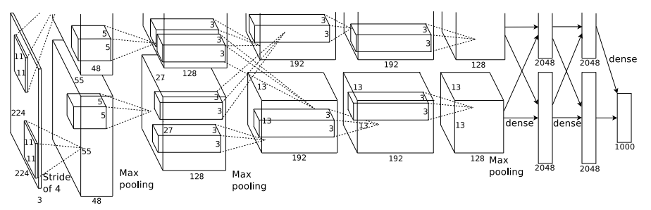
The paper introduces AlexNet, (though the term is not used in the paper), a CNN using 5 convolution layers + 3 Fully
Connected layers arranged in 2 parallel streams with limited cross-feeding, that improved the top-5 error rate on
ImageNet by a whopping 11% – from 26.2% to 15.3%. (Compare this with
the ResNet paper
2Deep Residual Learning for Image Recognition
He et al. CVPR 2016
See our review of this paper.
that got comparable Top-1 error rates.)
Within are details of the architecture and training. Though CNNs are a standard architecture today, this paper
also introduced, or was a very early adopter of, several other common architecture and training features, such as data
augmentation, max pooling, multi-GPU training, layer normalization, dropout, weight decay, categorical cross-entropy
loss, and ReLU nonlinearity. It also describes several other that are not as common any more, such as a color noising scheme
based on a PCA decomposition of the RGB space over all training inputs, a partial bifurcation of channels between two
GPUs, (model parallelization), an initialization strategy for the bias units, and an inference-time strategy of
evaluating on different crops of the test image and taking a vote from among the resulting predictions. This paper is
packed to the gills with innovations and that’s an important context when asking why Deep neural learning
didn’t really take off until it appeared.
Architecture
Their convolutional kernels at the first level are 11x11, which is rather large by recent standards.
Their multiple-GPU scheme is highly customized. They put half of the convolution channels on each GPU, but, layers 1 and 3 take inputs from both GPUs, while 2, 4 and 5 remain specific to the channels that are locally available. They used cross-validation to choose which layers take inputs from both GPUs vs. only locally. They used 50% dropout on the two hidden FC layers.
Indispensable implementation details
As mentioned above, this paper introduces a lot of implementation details that are indispensable for getting a DNN to work effectively. So let’s go through them one by one.
ReLU
The Rectifying Linear Unit (ReLU) (or its
younger siblings, the
Leaky ReLU
3Rectifier Nonlinearities Improve Neural Network Acoustic Models
Maas et al. ICML 2013,
GELU
4Gaussian Error Linear Units
Hendrycks\, Gimpel Arxiv 2016, etc. etc. etc.,)
is now the de-facto standard non-linearity in Deep Learning. The one thing that needs to be said about ReLU is that it
doesn’t “saturate”5“Saturating” is where the activation has an asymptotic maximum, and the output at some unit is very close to it.
When this happens, gradient updates that need to reduce that unit’s output get “stuck” because when a non-linearity is
already outputting near its asymptotic limit, it takes a massive gradient update to its inputs to decrease it. But, its
suppressed magnitude also suppresses the gradient, meaning that a single gradient update won’t materially
reduce its output. The Glorot paper below talks about this..
The paper does mention an earlier
Hinton paper
6Rectified Linear Units Improve Restricted Boltzmann Machines
Nair\, Hinton ICML 2010
To give an idea of how far back this is, the Hinton paper that introduced the ReLU was about fixing Restricted
Boltzmann Machines. that originated ReLU
units, but they were still new enough to warrant a few paragraphs to describe and motivate using
them over the previously common
sigmoid or
tanh.
Moreover, this paper rightly recognizes their importance – Section 3 (The Architecture) is ordered by the authors’
assessment of decreasing importance, and they put ReLU first.
One interesting observation is made in passing – when comparing with an earlier work that claimed tanh worked well, they point out that on the smaller Caltech-101 overfitting matters more than fast learning. So, it’s not so much that ReLU is always better than saturating functions, as it is more eager and regularizes less.
Lateral Inhibition
Their layer normalization is also highly customized, and imposes a kind of locality among channels. It’s a bit of a misnomer to call it “layer normalization” because each channel’s output is not normalized over the entire set of channels at the layer, but rather over a sliding window of channels. They found that a window size of 5 worked best. This is a particularly radical move because it disrupts the equivariance of almost all neural net units to reordering of the units.7That is, you can scramble the order of hidden units in any Fully Connected layer and get the same DNN. The same goes for channels in a Conv unit, or an LSTM or Transformer. Instead, this normalization scheme imposes local interactions that implement a kind of lateral inhibition inspired by real neurons. They report a drop of 1.4 %-point in top-1 error with this trick.
One might think of this not as a “normalization” trick, but as a joint activation function.
Dropout
This paper wasn’t the first
8Improving neural networks by preventing co-adaptation of feature detectors
Hinton et al. arxiv 2012
This one may or may not be the first to do something similar, but it does have to define the term “dropout”.
to use dropout, but it was close. Since Krizhevsky was in Hinton’s lab at the time, that explains where it came from.
Since dropout was such a new thing at the time, the paper even provides an explanation for why they’re using it
and what effect they expect it to have. The paper describes it as a kind of virtual ensemble method. Under this
interpretation, the average output of the model, (under different realizations of dropout,) is effectively an ensemble
of individually weaker classifiers, and see also the inference time voting scheme below. They report that using dropout
roughly doubles the training time, but who’s counting when you’re winning contests?
Categorical Cross Entropy
For classification in DNNs, you almost always use the Categorical Cross Entropy loss without ever thinking about it. It’s yet another unsung hero of modern Deep learning. Prior to this, it wasn’t unheard of for there to be a whole paper about some bespoke loss function and optimization scheme for dealing with Multi-class classification. Now, it’s common to do classification tasks with tens of thousands of classes and no one bats an eye. This paper does not use that terminology, and instead describes it as,
Our network maximizes the multinomial logistic regression objective, which is equivalent to maximizing the average across training cases of the log-probability of the correct label under the prediction distribution.
Compare this with the equation for Categorical Cross Entropy:
\[H(p, q) = -\sum_{x} p(x)\log q(x) \]
where \(p(x)\) is the class probability of \(x\), (which is uniform by default in all implementations I know of,) and \(q(x)\)
is the softmax output.
Data augmentation
Data augmentation is yet another indispensable step in modern Deep Learning. The term “augmentation” doesn’t mean “adding features” so much as “multiplying the size of your training set by adding perturbed examples”, so long as the perturbation is believed to not affect the label. Their data augmentation scheme is to take a random 224x224 patch from within the 256x256 input, and reflect horizontally at random. Like everything else, this was clever then, standard now.
They also did a colorspace manipulation trick that makes a lot of sense, but that I haven’t seen or heard much of since then – compare with this list of torchvision methods. The idea is to do PCA of the data in RGB space. That is, treating every pixel as a sample point in RGB space, presumably for all 78.6 billion pixels, they mean-centered them and computed a 3x3 covariance matrix, and then extracted its eigenvectors. For each new image they draw 3 random scaling coefficients \(\alpha_{1..3} \sim \cal{N}(0, 0.1)\), scale each eigenvector \(v_i\) by the corresponding \(\alpha_i\) and add it to every RGB pixel value in the image. This is a crude, but effective, way of altering the lighting of each image without drastically altering its appearance. Oddly, the paper doesn’t show what the eigenvalues are, nor what the 3 eigen-colors are, but one must assume they are meaningful because by itself this trick got them yet another %-point of error reduction.
Inference time voting
The paper uses the augmentation scheme in another way – at inference time, it takes 5 crops, with and without horizontal flipping, for 10 in total. Then it averages the outputs across all. Where an ensemble averages across multiple realizations of the training process, this data augmentation averages across multiple realizations of the feature vector. I’ve seen at least one other paper since then that re-invented this trick, and it is an effective one. But with all of the other novelties in this paper it seems to have been lost in the shuffle.
Learning rate schedule
They used a clever-then / standard-now learning rate schedule wherein every time validation error leveled out, they dropped the learning rate by 10x. Nowadays pytorch has a host of learning rate schedulers, and keras has hooks for rolling your own, but at that time all of this was hand made.
Initialization scheme
At last the paper has one archaism – they used a 0-mean Gaussian distribution for random initialization, rather than the
now-common
Glorot scheme
9Understanding the difficulty of training deep feedforward neural networks
Glorot & Bengio AISTATS 2010
The essence of the Glorot initialization is for the variance of the weights to be scaled by both the size of the current
layer and the next one. That seems to be a sufficient condition for activations’ variance to be comparable between one
layer and the next, which is a necessary condition for gradients to propagate well. Having bounded support doesn’t seem
to be necessary, though most implementations I’m aware of have it. Tensorflow has a clipped Gaussian that they call
Glorot Normal, whereas
pytorch has both a
plain uniform distribution like
eq. (1) in the Glorot paper, and a
normal distribution
as well., which is a Uniform distribution.
For the biases, however, they had yet another novel scheme. Recalling that in the 2-GPU scheme, the 2nd, 4th and 5th convolutions only take input from the stream on the same GPU, while the 1st and 3rd takes input from both. The first set had their biases initialized to 1, while all others were initialized to 0. They claim this speeds up learning in the early iterations since effectively all neurons are getting gradient updates rather than being suppressed. They don’t say why this is preferable only in the layers that don’t take input from both GPUs.
Max pooling
They reference earlier sources regarding max-pooling, however they pool with overlapping fields, which gives a 0.4%-point bump in top-1 accuracy.
Multi-GPU model parallelization
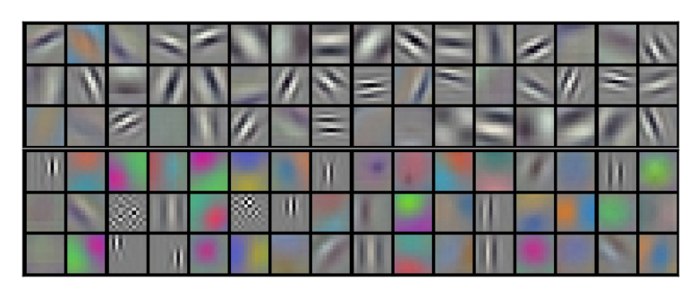
Model parallelization is of course alive and well today, but it’s much less common to see any bespokeness to how it’s implemented10Or maybe it is and I’m just missing out???. However, the implications of having each branch only take inputs from one branch are interesting. The paper notes that in every run that they did, one GPU always learned (mostly) color invariant features, which resemble Haar wavelets, while the other would learn color sensitive patterns like blue-yellow or red-green gradients. It is a bit maddening that the paper notices this, and then just says “huh” and moves on.
They report yet another decrease of 1.7%-points in top-1 test error over a 1-GPU scheme with about half as many convolutional channels as for the 2-GPU scheme.
Discussion
There aren’t many limitations to discuss because the task they’re doing is very simple, and well understood. They do mention that they expect results to improve with more GPU power, which has largely been borne out since then. They also mention that they didn’t do any unsupervised pre-training, again due to only having 2 GTX 580 GPUs to work with.
They also show a few examples of how all or most of the top predictions for several sample images are reasonable mis-classifications, i.e. falling within a broader category of animals or household objects as the true label. They also show several sets of input images that are extremely close together in the late-stage latent space, and sure enough they strongly resemble one another in subject matter, but are not near to one another in a pixel-wise \(\ell_2\) sense.
So that’s the paper. What did I take away from it?
- This is very bespoke setup, which is masked by the fact that several of the ideas within are now ubiquitous. It’s much more common to see the occasional flourish in a model that’s often the result of endless tinkering as opposed to a narrowly focused abstract idea.
- This paper came from Hinton’s lab, which is why it was so early to adopt several of its most effective tricks. Like other Hinton lab papers, there’s a healthy does of inspiration from neuroscience. E.g. the neural column-like design of the convolution net or the lateral inhibition inspiration for the normalization scheme, or the idea behind dropout.
- On the other hand, while it has new ideas and deep ideas, it doesn’t have all that many new, deep ideas.
- In spite of there being so many now-ubiquitous practices in this paper, there are a few novel ones that may deserve another chance. I’m most intrigued by the sliding window approach to normalization. Given that Batch normalization is a standard practice now, and how much of a problem you’ll have without some kind of normalization strategy, it’s clearly important to control the magnitude and variance of outputs at each layer, but relaxing that in such a way as to allow for some kind of structural invariance to emerge could also be interesting. Their color-space noising scheme seems especially promising too. The inference time voting trick has been seen elsewhere, but not as often as it probably should.
- The paper does a very good job of making an ablation study11I.e. where the innovations are removed one at a time to see which one had the most impact, and so on. of its innovations. It doesn’t do so for all, since there are so many, but it is very useful indeed seeing a ranked list of which tricks were the most effective.
Final thoughts
This paper demonstrates an instance of a phenomenon wherein for some tasks there turns out to be a set of necessary components, practices or conditions that have to be met before you can start to really succeed. It’s an unfortunate situation to be in because it means you can be making steady progress and yet not show any major improvement. Then one day you cross some invisible threshold and suddenly all of the lights come on. I don’t doubt that for all of the tricks they pulled from other papers there was evidence that they were working on their own, but what made AlexNet special was just how staggeringly well all of these ideas work when put together in concert.
Comments
Comments can be left on twitter, mastodon, as well as below, so have at it.
Our first post!
— The Weary Travelers blog (@wearyTravlrsBlg) April 23, 2023
Paper review: The AlexNet paperhttps://t.co/dmzgu38ZeO
To view the Giscus comment thread, enable Giscus and GitHub’s JavaScript or navigate to the specific discussion on Github.
Footnotes:
Note that there is another paper by the same authors in Communications of the ACM 2017, with exactly the same title, except that it has over 130,000 citations. We are reviewing the original 2012 NeurIPS paper here, which is basically the same paper.
Deep Residual Learning for Image Recognition
He et al. CVPR 2016
See our review of this paper.
Rectifier Nonlinearities Improve Neural Network Acoustic Models
Maas et al. ICML 2013
Gaussian Error Linear Units
Hendrycks\, Gimpel Arxiv 2016
“Saturating” is where the activation has an asymptotic maximum, and the output at some unit is very close to it. When this happens, gradient updates that need to reduce that unit’s output get “stuck” because when a non-linearity is already outputting near its asymptotic limit, it takes a massive gradient update to its inputs to decrease it. But, its suppressed magnitude also suppresses the gradient, meaning that a single gradient update won’t materially reduce its output. The Glorot paper below talks about this.
Rectified Linear Units Improve Restricted Boltzmann Machines
Nair\, Hinton ICML 2010
To give an idea of how far back this is, the Hinton paper that introduced the ReLU was about fixing Restricted
Boltzmann Machines.
That is, you can scramble the order of hidden units in any Fully Connected layer and get the same DNN. The same goes for channels in a Conv unit, or an LSTM or Transformer.
Improving neural networks by preventing co-adaptation of feature detectors
Hinton et al. arxiv 2012
This one may or may not be the first to do something similar, but it does have to define the term “dropout”.
Understanding the difficulty of training deep feedforward neural networks
Glorot & Bengio AISTATS 2010
The essence of the Glorot initialization is for the variance of the weights to be scaled by both the size of the current
layer and the next one. That seems to be a sufficient condition for activations’ variance to be comparable between one
layer and the next, which is a necessary condition for gradients to propagate well. Having bounded support doesn’t seem
to be necessary, though most implementations I’m aware of have it. Tensorflow has a clipped Gaussian that they call
Glorot Normal, whereas
pytorch has both a
plain uniform distribution like
eq. (1) in the Glorot paper, and a
normal distribution
as well.
Or maybe it is and I’m just missing out???
I.e. where the innovations are removed one at a time to see which one had the most impact, and so on.