We’ve covered the motivation, so now it’s time to dig in to the algorithm itself. Here is the listing from the paper itself:

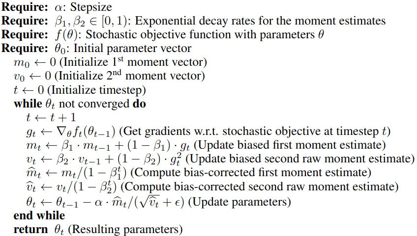
So what’s happening here? We need a Step size \(\alpha\), two \(\beta\) hyperparameters between \(0\) and \(1\), a function \(f\) to minimize with parameters \(\theta\) and an initial guess \(\theta_0\). Given that you already need \(f\), \(\theta\) and \(\theta_0\) in order to do SGD, we end up with three parameters that we actually care about. Also, in practice, it is very unlikely that you’ll need to tinker with the \(\beta\) hyperparameters, so it really just comes down to this \(\alpha\). Note that they call it a “Step size”, rather than a “Learning rate”, but it functions the same way that a learning rate does in other algorithms. Nevertheless, the paper claims that an advantage of Adam is that the step size really is close to a true step size, or at least it bounds the true step size⁵⁵It’s important to remember that this “step size” is an element-wise bound on the amount by which any element can change, rather than the magnitude of any whole step..

Next: what state does it keep track of? There are not one, but two momentum vectors, \(m_t\) and \(v_t\), and of course \(t\) is just an iteration counter. The main flow of the algorithm is to,

• Compute a negative cost gradient \(g_t\). This includes all regularizers such as L1 or L2; dropout; and any other gradient noising.
• Update the momentum \(m_t\) by taking a weighed average between \(m_{t-1}\) and \(g_t\). The weight is heavily in favor of the momentum \(m_t\). This is controlled by \(\beta_1\), and given a default value of \(0.9\), it’s pretty heavily weighted towards preserving the momentum, which is the point of momentum.
• Update the squared momentum \(v_t\) by taking a weighted average between \(v_{t-1}\) and squared gradient \(g_t^2\). Once again the weight, controlled by \(\beta_2\) is very heavily weighted towards preserving the momentum, with a default value of 0.999.
• Rescale the two momentum terms by dividing them by \(1 - \beta^t\), where \(\beta\) is the corresponding parameter used above. Note that it is taken as a power of \(t\). At first this means dividing the momentum terms by something small, which will blow them up, but relatively soon the algorithm will be dividing them by something close to \(1\).
• Finally, do the update. As with SGD with momentum, we add the momentum term to \(\theta\), not the gradient, scaled by the step size \(\alpha\). But here is where Adam differs – the update is also divided by the element-wise root of the squared momentum term \(v_t\).

Clearly Adam differs from SGD by keeping track of a squared momentum term. It uses the squared momentum to figure out what the appropriate step size ought to really be, hence the name. We could think of this as a poor-man’s Newton’s method. In Newton’s method, we compute the entire Hessian matrix of the objective, invert it, multiply the gradient by it, and then proceed with the update. This is doing something similar, except that it only uses the diagonal, and a squared gradient rather than the true second derivative⁶⁶Note that the diagonal of the Hessian is not the same as the squared gradient, however, according to eq. 8 of this early LeCun paper, this is the “Levenberg-Marquardt approximation”.
Optimal Brain Damage
LeCun et al., NeurIPS 1989
These course notes give a slightly different explanation.. Considering that the inverse of a diagonal matrix is computed by taking the inverse of the diagonal elements, we could technically consider this as an approximate second order method.

It’s also worth noting that the division of \(\hat{m_t} / \hat{v_t}\) is done element-wise, meaning that the step is scaled independently for each element of \(\theta\), which is why the paper claims that it is adaptively scaling the step size for each element⁷⁷Compare with the method used in:
Visualizing the Loss Landscape of Neural Nets
Li et al., NeurIPS 2018
See our outline of this paper..

Lastly note the term \(\epsilon\). That’s not a true hyperparameter, since its value should be determined not by the characteristics of \(f\), but by the numeric type of \(\theta\), i.e. \(32\) bit or \(16\) bit float, or whatever. The pytorch version of Adam has a default value of \(10^{-8}\). The keras version uses \(10^{-7}\).

The method devotes a whole step to rescaling \(m_t\) and \(v_t\). The paper explains that this is because it uses \(0\) as an initial guess, and the initial steps of blowing up the two moments are just there to get it away from \(0\), which is a biased initial guess. Almost any initial guess would likely be biased, or at any rate it would contain much less information about the objective function \(f\), so it makes sense to front load the moments heavily with early gradient updates, and smoothly bring them back down to the un-corrected version.

The paper argues that the ratio \(\hat{m_t} / \sqrt{\hat{v_t}}\) is conceptually like a Signal to Noise Ratio (SNR). That is, when there is a large first moment, and not much second moment, estimated over a decaying window, then there is sufficient evidence to take a larger step (relative to the gradient size!) It makes sense that if the recently observed momentum from gradient steps is larger than the root-mean-squared gradient from a much longer history, then a bolder step should be taken. This means it’s doing something like a relaxed – or adaptive – Trust Region method.

The paper then offers another explanation. What we really want is an estimate of the squared gradient \(g_t^2\). However, what we really get is this \(v_t\) thing that is an average over an exponential window: \[ v_t = (1 - \beta_2) \sum_{i=1}^t \beta_2^{t-1} \cdot g_i^2. \] The paper then gives this derivation:

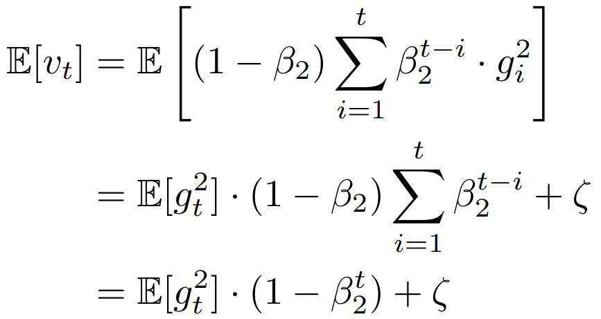
The extra \(\zeta\) term is just an accounting for “non-stationarity” of \(g_t\), i.e., anything that varies as a function of \(t\), apart from the first term. It should just be ignored, because just by using a gradient method with momentum we’re already ignoring it. The last line basically shows that in expectation, \(v_t\) is \((1 - \beta_2^t)\) times \(g_t^2\). Perhaps the simplest way to think of it is that when taking a weighted window average, the coefficients should sum to \(1\)! The last line of this equation is telling us that the coefficients actually sum to \((1 - \beta_2^t)\), so we should divide by that sum to correct for it.

An optimization method is no good if it doesn’t ultimately converge, and the paper provides a justification for why it does. The argument goes by borrowing regret-bound machinery from elsewhere. Regret is a concept from online learning where we compare the sum total of the errors of a model that learns from one example at a time against the error of the best model we could have trained if we had had all of the data up front. Here, the idea is to compare the error of all of the \(\theta_t\) iterates against the optimal \(\theta^*\), which can be posed as a regret bound. The appendix has a proof showing that the regret is bounded by \(O(\sqrt T)\).

The main theoretical result makes the following assumptions:

• The function \(f_t\) has bounded gradients: \(\|\nabla f_t(\theta)\|_2 \le G, \|\nabla f_t(\theta)\|_\infty \le G_\infty\). In other words, both the magnitude, and the largest element have a maximum size.
• The distance between successive iterates is bounded: \(\|\theta_n - \theta_m\|_2 \le D, \|\theta_n - \theta_m\|_\infty \le D_\infty\), for any time steps \(m, n\). In other words, there is both a spherical radius that Adam never leaves, and also a largest element-wise divergence between any pair of iterates.
• \(\beta_1^2 < \sqrt{\beta_2}\). This is pretty easy because in practice you usually want \(\beta_1 < \beta_2\). As before, both have to be between \(0\) and \(1\), which means \(\sqrt{\beta_2}\) is actually larger than \(\beta_2\).
• The learning rate \(\alpha\) decreases over time, such that \(\alpha_t = \alpha / \sqrt{t}\).
• \(\beta_1\) also has a decay schedule: \(\beta_{1, t} = \beta_1 \lambda^{t-1}\), for some \(\lambda \in (0, 1)\).

The first is pretty easy to assume, as long as your loss function is reasonably well behaved. The third is true by default, and basically says undefined behaviors are the fault of the operator. The second one is a bit of a crutch. Taken literally, it basically says, “In order to prove that Adam converges, we need to assume that it will never leave some bounded region of \({\mathbb R}^d\).” So what they’re proving is that so long as it doesn’t shoot off to infinity, it will settle down. It should suffice to show that there is a maximum step size that can be taken in any event, but it probably won’t improve the paper to show that, so they just assume it.

The fourth is interesting because in practice one might actually not do that, yet Adam still happily converges. The fifth is… not totally bonkers, but it’s also not common practice, at least not that I’ve ever heard of. Nevertheless, the paper says,

Decaying \(\beta_{1,t}\) towards zero is important in our theoretical analysis and also matches previous empirical findings, e.g. (Sutskever et al., 2013)⁸⁸On the importance of initialization and momentum in deep learning
Sutskever et al., ICML 2013 suggests reducing the momentum coefficient in the end of training can improve convergence.

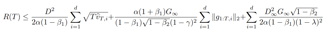
The result itself is a monster equation with the regret \(R(T)\) in the LHS, with several \(D^2\), \(D_\infty^2\), and \(G_\infty\) terms on the right. It also features a sum of 2-norms of single gradient elements over time, so if we think of a gradient as a column of a matrix that has \(T\) columns, one for each time step, then the row norms of this matrix play a part in the result. That’s the \(\|g_{i:T,i}\|_2\) term. The paper claims that when there are sparse gradients, this term will be lower, which is why they claim Adam works well on sparse gradients. Of course, this is a bound so how typical is it…?

Here it is in all its gory detail:

The paper devotes a whole section to comparing Adam with several existing algorithms, RMSprop and AdaGrad.

RMSProp⁹⁹Divide the gradient by a running average of its recent magnitude
Tieleman and Hinton; Coursera: Neural networks for machine learning, Lecture 6.5
Yes, that’s how this paper cited RMSProp.

The paper explains it quite nicely.

RMSProp with momentum generates its parameter updates using a momentum on the rescaled gradient, whereas Adam updates are directly estimated using a running average of first and second moment of the gradient. RMSProp also lacks a bias-correction term; this matters most in case of a value of \(\beta_2\) close to \(1\) (required in case of sparse gradients), since in that case not correcting the bias leads to very large stepsizes and often divergence

AdaGrad¹⁰¹⁰Adaptive Subgradient Methods for Online Learning and Stochastic Optimization
Duchi et al., JMLR 2011
The paper gives this update rule for AdaGrad: \[ \theta_{t+1} = \theta_t - \alpha \cdot g_t / \sqrt{\sum_{i=1}^t g_t^2}. \] In other words, there is no window decay, or equivalently \(\beta_1 = 0\) and \(\beta_2 = 1\), and \(\alpha_t = \alpha\cdot t^{-1/2}\). What’s interesting is that this is equivalent to Adam, specifically with the bias correction terms. Without them, this would be numerically unstable.

The experiments focused on showing that Adam converges faster than other methods. To facilitate comparison, the same random initialization was shared across all methods, and a hyper-parameter grid search was done separately for all methods with the best results being reported for each. The models they examined ranged from tiny, (a simple logistic regression MNIST / IMDB model,) small, (a multilayer perceptron MNIST classifier,) and medium-sized by the standards of the time, (a plain convolutional CIFAR10 classifier).

The paper has an odd zinger at the end – temporal averaging. That is, the paper makes a last minute proposal, after all of the experiments are done, to try averaging the weights over several update steps. This can be done uniformly over the entire training run, or with an exponential decay favoring more recent updates. This trick does work, though as a form of momentum it has to be used carefully¹²¹²On the importance of initialization and momentum in deep learning
Sutskever et al. ICML 2013
. I’m aware of at least one successful use case.